2. Measure IID H∞
Golden Equation 2 - measure $H_{\infty}$ only when samples are IID
Peter Drucker said “If you can’t measure it, you can’t improve it.” Very true. So you need to measure the entropy being generated by the observer. You have to realise that actually there is no such thing as a hardware random number generator, unless you’re thinking of a roulette wheel. This can be easily proven with simple experiments. Take a commercial USB sized TRNG. Hold one up and then caress it. Do random bits spurt emerge in a stream of unpredictable ones and zeros? No? Or stare at a Zener diode. Do you see entropy? No?
More specifically, unless you’re operating a roulette wheel or bits are delivered to you from on high carved into stone tablets, all random numbers are software generated after observations of a physical process. After all a bit is software so has to be made by software. As hardware begets hardware, so software begets software. It’s just a question of the relative proportions of software and hardware and the rate and resolution that one samples the other.
Given the shenanigans with NIST SP 800–90B, BSI AIS 20/31 and real world inappropriateness of the ubiquitous (and often misunderstood) Shannon log formula when applied to the general case, we suggest de-correlating the sampling regime to obtain independent and identically distributed samples. De-correlate, de-correlate, de-correlate. It’s way more certain and thus more secure.
$(\epsilon, \tau)$-entropy per unit time
This is what it’s all about. The degree of dynamical randomness of different time processes can be characterized in terms of the $(\epsilon, \tau)$-entropy per unit time. The $(\epsilon, \tau)$-entropy is the amount of Kolmogorov information generated per unit time, at different scales $\tau$ of time and resolution $\epsilon$ of the observables. This quantity generalizes the Kolmogorov—Sinai entropy per unit time from deterministic chaotic processes, to stochastic processes such as fluctuations in physico-chemical phenomena or strong turbulence in macroscopic space time dynamics[1]. Although we do have to append our standard stability clause here.
Or more completely, what we seek to measure when the entropy samples are proven to be IID. An information theoretical upper bound on the entropy rate is given by the Shannon-Hartley limit (theoretical upper limit for rate of information transfer in a system with a given bandwidth)[2]:-
$$ H(\epsilon, \tau^{-1}) < H_{SH} = 2 BW \times N_{\epsilon}$$
where $N_{\epsilon}$ is the number of bits per sample that the digitizer(ADC) measures at a given measurement resolution $\epsilon$, sample rate $\tau^{-1}$, and $BW$ is the bandwidth of the signal measured by the digitizer. $BW$ is limited by the analogue bandwidth of the physical entropy source as well as the digitizer and associated circuitry such as transistors, amplifiers and comparators. The above equation gives the maximum rate at which information can be obtained from the signal by the digitizer. Of course, the equation overestimates the upper bound because the effective bandwidth is often less than the standard signal bandwidth [3] and the effective number of bits of a digitizer is often less than the stated number of bits [4].
Importantly, what we find as a rule of thumb is that for real world (limited bandwidth) stochastic entropy sources :-
$$ \begin{array}{l} \text{As } \epsilon \to 0, H \to \infty \text{ and } R \to 0 \\ \text{As } \tau \to 0, H \to 0 \text{ and } R \to 1 \\ \end{array} $$
where $R$ is normalised autocorrelation. So the moral of this story is that faster is not necessarily better, as autocorrelation will punish you. Which is all better shown with pictures of signal sampling:-
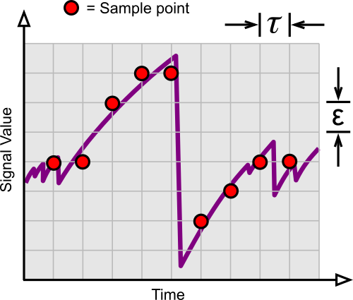
Correlated (non-IID) data samples with a small $\tau$.
You can see that the above samples follow the uphill signal (characteristic of a Zener diode in avalanche). They are highly autocorrelated.
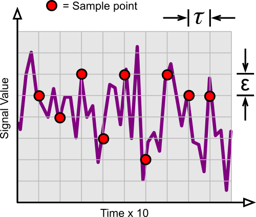
Uncorrelated (IID) data samples with a large $\tau$.
In this case, the samples are not autocorrelated as the sample interval $\tau$ has been increased ten fold. That is what we are trying to achieve.
A simpler example with dice

In this example, imagine a fair pair of dice that drop out of the sky every second. And then imagine if we observe the pair and count the pips every two seconds. In this image we count three, but the next number of pips is unknown until the next pair of dice fall and we count them again. We can guarantee that the next count will be completely independent of the first count as the dice are falling faster than we’re observing them $(R = 0, H_{\infty}/ \text{Sa} = 2.58 $ bits). Now imagine if we decide to increase the observation rate to ten counts per second. It is apparent that at least nine of our observations will count exactly the same number of pips as we’re observing faster than the dice are falling. Thus we have a very strong correlation between counts $(R \approx 1, H_{\infty}/ \text{Sa} \approx 0$). The observations are not independent; they are loads correlated and the entropy rate vastly diminished.
How to ensure IID sampling
By following the following flowchart:-
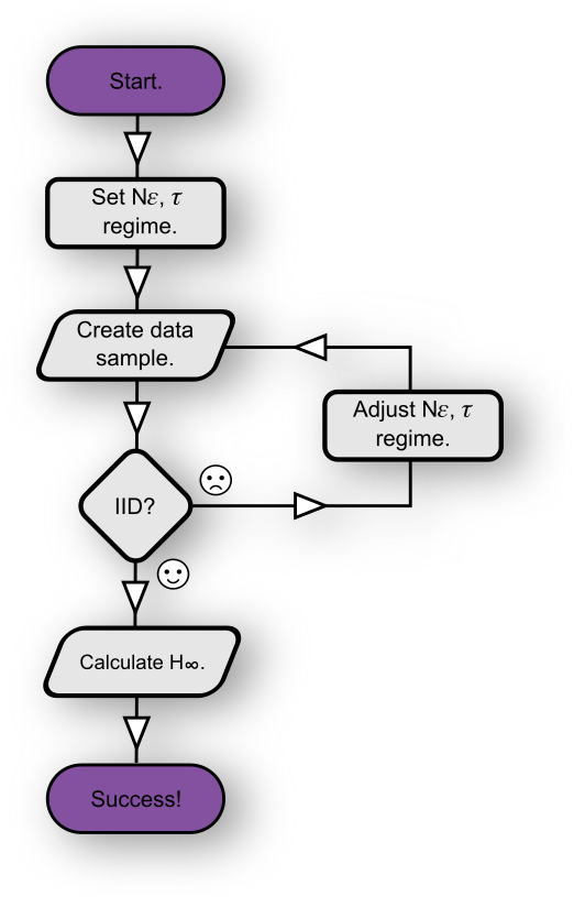
How to set $N_{\epsilon}, \tau$ to ensure IID sampling.
You can test for IIDness via one or all of the available IID tests; our fast test, our slow test or NIST’s SP800-90b ea_iid test. And by adjusting $N_{\epsilon}, \tau$, we mean that you either slow down the sampling $(\tau \uparrow)$ or discard some of the sample bits $(N_{\epsilon} \downarrow)$. Realistically increasing sample resolution $(\epsilon)$ is harder. You may need to upgrade the ADC used, or easier, it may be possible to lower the reference voltage $(\epsilon \downarrow)$. This is quite easy for Arduino/Atmel AVR based devices. Decimating the samples is an equivalent alternative to increasing the sample interval, i.e. ignore every say 2nd/3rd/4th e.t.c sample. There are examples (ring oscillators) where the decimation ratio is 1 : 500 or even more!
How to actually measure $H_{\infty}$
Now that you have generated a provably IID sample file (with appropriate $N_{\epsilon}, \tau$ settings), there are three methods:-
-
If you used NIST’s
ea_iidprogram, you just read $H_{\infty}$ from a line looking likemin(H_original, 8 X H_bitstring): 7.947502. -
If you used
entwith the-cargument, pick the most common value from a line looking like220 � 22322185 0.223222and calculate $-\log_2 (0.223222)$. -
Or estimate the largest probability value from a probability mass function/ histogram, then do the $-\log_2 (p_{max})$ thing as above.
And so there we have it, $H_{\infty}$ with very good certainty.
References:-
[1] Pierre Gaspard and Xiao-Jing Wang. Noise, chaos, and (ε, τ )-entropy per unit time. Physics Reports, 235(6):291–343, 1993.
[2] Emmanuel Desurvire. Classical and quantum information theory: an introduction for the tele- com scientist. Cambridge University Press, 2009.
[3] Fan-Yi Lin, Yuh-Kwei Chao, and Tsung-Chieh Wu. Effective bandwidths of broadband chaotic signals. IEEE Journal of Quantum Electronics, 48(8):1010–1014, 2012.
[4] Robert H Walden. Analog-to-digital converter survey and analysis. IEEE Journal on Selected Areas in Communications, 17(4):539–550, 1999.